Three years is a useful horizon for a blade forecast: long enough to align with a procurement or capital cycle, and short enough that the assumptions still look like something a fleet recognises. The forecast itself comes from one base input — the consumption history per machine — with every other factor applied as an adjustment to it rather than as a replacement for it.
This is the implementation path for building that document: assembling the base input, adjusting for fleet change and winter severity, stating the price and lead-time assumptions separately, and presenting the result in a form a budget committee can act on.
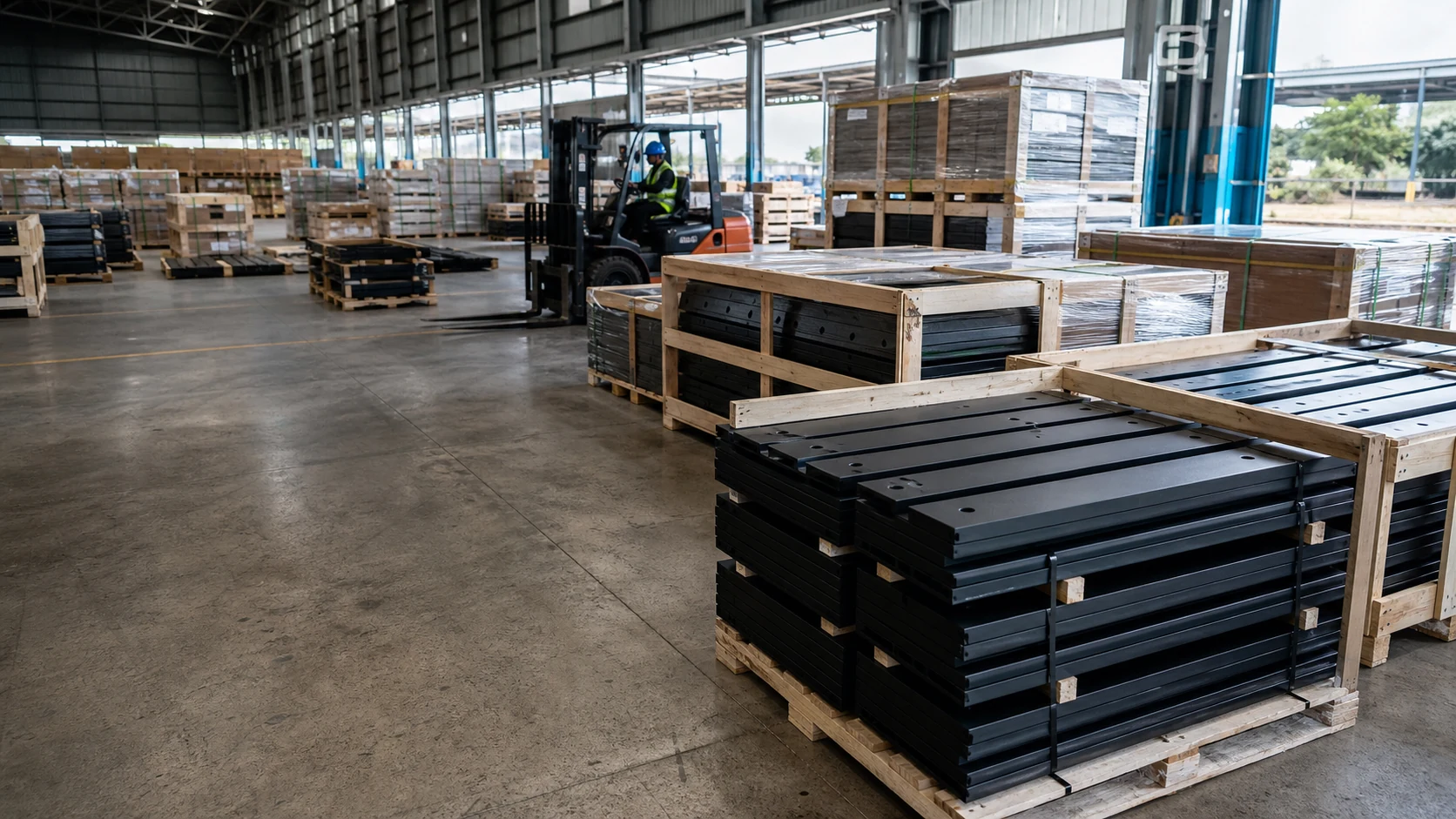
Plow blade procurement forecast: what the forecast is for
A forecast sets a quantity and a budget.
A procurement forecast is not a prediction of the winter. It is a statement of what the fleet expects to consume, on stated assumptions about the weather and the fleet, so that a quantity can be bought and a budget set.
That framing determines what belongs in the document: a base case, the adjustments applied to it, and enough disclosure that a reader can disagree with one assumption rather than with the whole figure.
Two properties make such a document useful. It has to be traceable, so that each year’s actual consumption can be compared with the forecast that was made for it. And it has to be adjustable, so that a change in the fleet or in the price assumption can be applied without rebuilding the model.
Consumption history as the base input
Consumption history is the only part of the forecast that rests on measurement, so it should be the most detailed. The useful form is consumption per machine per season, expressed in a unit that can be compared across winters — events, lane kilometres or blade-down hours rather than months.
Three refinements make the history usable. Recording consumption by machine rather than by fleet, because a small number of units usually drive the total and a fleet average hides them. Recording the route each machine worked, so that a route change can be reflected rather than discovered. And recording the edge specification fitted, because a specification change alters consumption and will otherwise appear in the history as an unexplained step.
Where a fleet has less than two seasons of usable history, the first year of the forecast is inevitably an estimate. That is a reason to start recording immediately, not a reason to postpone the forecast.
Fleet growth and vehicle changes
The fleet will not be the same in the third year as in the first, and three changes move the forecast. Machines added to the fleet add consumption in proportion to the duty they take on, which is not the same as the fleet average. Machines retired remove consumption, and their blades may be reusable on the machines that replace them, which reduces the new requirement. And route reassignments move consumption between machines without changing the total.
Those three are usually known before the forecast is written, because they come from the fleet’s own plan. Applying them as explicit adjustments, line by line, is what makes the forecast defensible; folding them into a general percentage increase is what makes it arguable.
Winter severity scenarios
Severity is the largest single uncertainty in the forecast, and the table below sets out how a fleet’s base consumption behaves under different conditions.
| Scenario | Effect on consumption | What it is used for |
|---|---|---|
| Mild winter | Fewer events and less abrasive contact | The lower bound, and the case that leaves stock unused |
| Average winter | The base case, taken from history | Budgeting the expected requirement |
| Severe winter | More events and deeper freeze, so higher wear and more damage | The case the fleet has to survive rather than plan for |
| Two severe winters in three | Total consumption rises across the horizon | Testing whether a three-year purchase should be sized higher |
The fourth row is the one that changes decisions. A three-year forecast built on three average winters is the arithmetic a fleet is comfortable with; the same forecast with two severe winters in it is the arithmetic that justifies carrying more stock or negotiating a volume position earlier. Winter maintenance research that supports these assumptions is published by the Transportation Research Board.
Price escalation assumptions
Price escalation belongs in the forecast and not in the consumption model. Stating it as a separate line, with the rate and the reason for it, allows a reviewer to change the rate without touching the quantity assumptions, which is what a finance function will want to do.
Two points about the assumption itself. A forecast that applies escalation only to the purchase price and not to freight or to any imported component understates the total, because those move too. And the choice between a single rate and a rate per year is less important than writing down which was used, so that the following year’s comparison knows what it is comparing against.
Volume purchasing and storage trade-offs
The forecast sets a quantity, and the quantity interacts with how it is bought. The table below sets out what a larger purchase moves.
| Element | Effect of buying the horizon in one order |
|---|---|
| Unit price | Improves where the volume is material to the supplier |
| Storage | Requires space for the whole horizon, off the floor and out of water |
| Obsolescence risk | Rises if the fleet changes specification before the stock is used |
| Working capital | Tied up earlier, which is a real cost even where the unit price falls |
| Supply risk | Falls, because the fleet holds what it needs for more than one season |
The third and fifth rows are the two that decide the question for most fleets. A procurement position taken for three years is a bet that the specification will not change, and it is a good bet on a standardised fleet and a poor one where machines are being replaced. How the specification itself is consolidated is covered on the blade standardisation page.
Presenting the forecast to council
A forecast that has to be approved by an elected body needs a different shape from a working model, and the sequence below produces one that survives the meeting.
- State the base case as a single quantity, with the consumption history it came from.
- Show the adjustments as named lines: fleet change, severity, and specification change.
- Present the severe-winter case alongside the base case rather than in an appendix.
- State the price assumption and the escalation rate as separate lines.
- State what the forecast does not cover, such as damage from a single event.
The fifth item protects the forecast more than it weakens it. A document that says what it excludes can be defended when something outside its scope happens; one that implies completeness cannot.
Review cadence
The forecast is reviewed on a fixed cadence rather than whenever the numbers look wrong.
- End of each season: compare actual consumption against the forecast for that year.
- Before each buying cycle: re-run the remaining horizon with the updated history.
- On a fleet or route change: apply the change to the remaining years rather than rebuilding.
- Annually: review the price and severity assumptions and record any change.
The first step is the one that improves the forecast. A fleet that compares its actual against its forecast each season learns where its assumptions are weak, and it usually finds that the consumption per machine is better than assumed while the severity assumption is worse.
What makes a forecast defensible
Three properties separate a forecast that gets approved from one that gets re-cut by a finance function.
- Every figure traced to a record, rather than to an estimate nobody can check.
- Assumptions stated separately from quantities, so they can be challenged individually.
- A severe case presented as a case rather than as a contingency line.
The third is the one that gets the quantity right. A contingency percentage applied to an average year is a number that satisfies a budget process and does not change what the fleet holds, whereas a severe case shows the reader what the fleet would actually need in the winter the forecast is meant to prepare for.
Common forecast errors
Four errors account for most forecasts that are revised mid-year. Building from a fleet average rather than per machine, which hides the units that drive consumption. Treating a route change as a percentage rather than as a reassignment between machines. Applying price escalation to the purchase price only. And sizing the forecast to the expected winter rather than to the winter the fleet has to survive.
Making the forecast a working document
A forecast that is written once and filed is an estimate; one that is updated each season with actual consumption becomes a planning tool. The difference between the two is a single habit — comparing the actual against the forecast at the end of the season and recording why they differed.
That comparison also feeds the fleet’s operational decisions rather than only its budget. Consumption per machine, once it is reliable, is the same figure the stock level and the specification review are built from, and the inventory side of that is described on the blade inventory planning page. Public sector budgeting practice is published by the National Association of Counties and the American Association of State Highway and Transportation Officials, network guidance by the Federal Highway Administration, and fleet practice by the Snow and Ice Management Association.
SENTHAI manufactures plow edges, wear plates and carbide inserts in Rayong, Thailand, and supplies fleets and distributors against a specified pattern, with lead times that depend on an order’s position relative to the season. Forecasts that need the specification and the supply position confirmed can be raised through the contact page.
FAQ
What is a plow blade procurement forecast based on?
Consumption history per machine, adjusted for changes in the fleet and for winter severity, with price and lead time assumptions stated separately. The history is the base input; everything else is an adjustment applied to it rather than a replacement for it.
How many years should a blade forecast cover?
Three years is a workable horizon: long enough to align with a capital or procurement cycle and short enough that the assumptions are still recognisable. Beyond three years the severity and price assumptions carry more of the number than the consumption history does.
Should a forecast use an average winter?
It should state one, and it should not be built on one alone. A single average hides the fact that a severe winter can double consumption, which is the scenario the fleet actually has to survive, so presenting a base case with a severe case alongside it is what makes the forecast usable.
How do price escalation assumptions affect the forecast?
They change the total but rarely the decision. What changes the decision is the consumption assumption, because a mild error there moves the figure by more than several years of escalation. Stating the escalation rate explicitly matters more than the rate chosen.
Send the consumption history, the fleet plan and the routes each machine works. The SENTHAI engineering desk will confirm the specification and the supply position so the forecast can be built against a lead time rather than an assumption.